Kalman Filters

I’ve spent the past week learning all I can about Kalman filters. The best description I found was:

the fundamental idea is to blend somewhat inaccurate measurements with somewhat inaccurate models of how the systems behaves to get a filtered estimate that is better than either information source by itself

At its essence, you take a prediction based from past data, take a prediction based on a bunch of observed variables, then combine the two to come up with an even better prediction.

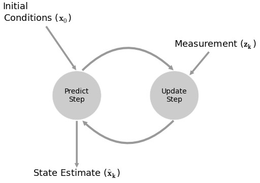
Everything is modeled with a linear system. There is a lot of matrix algebra, covariance matrices, maximum-likelihood estimates, and fancy math. I’m not going to go into the details, but you can learn more below in my presentation.

Application

I estimated the beta of the VIX using pykalman and compared it to the 30 day, 1 year, and 2 year rolling betas. All parameter fitting was done using walk forward optimization. I then used the model results to simulate hedging future VIX movements.

Below are my results.

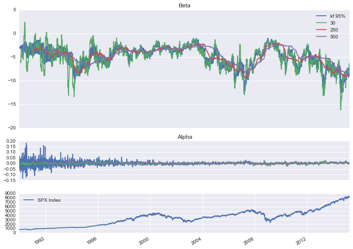
The blue area in the top two graphs are the 95% confidence intervals for the parameter estimates. As you probably notice, the rolling betas are always several steps behind. The Kalman filter is quick to adapt to new information, but also successfully filters out the noise.

Below is graphical analysis of the errors for the Kalman filter. Normal. Stationary. Homoscedastic. Check. Check. Check.

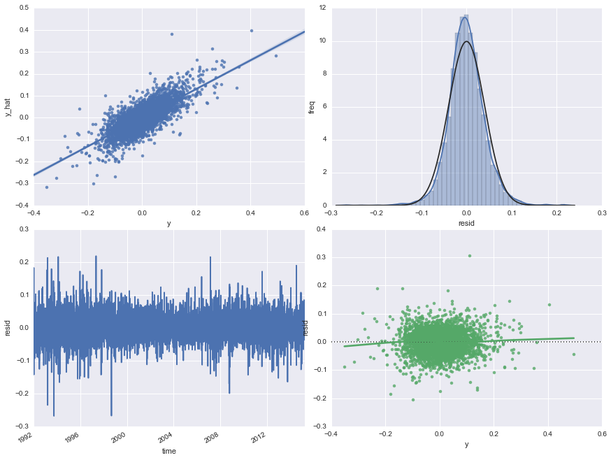
At the end of the day, what we can really care about is prediction accuracy, and indeed, Kalman filters outperform all rolling betas in terms of mean squared errors.

Check out the rest of my presentation here.